Subtitles & vocabulary
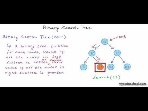
Data structures: Binary Search Tree
00
Hhart Budha posted on 2014/06/15Save
Video vocabulary

sort
US /sɔrt/
・
UK /sɔ:t/
- Transitive Verb
- To organize things by putting them into groups
- To deal with things in an organized way
- Noun
- Group or class of similar things or people
A1TOEIC
More time
US /taɪm/
・
UK /taɪm/
- Uncountable Noun
- Speed at which music is played; tempo
- Point as shown on a clock, e.g. 3 p.m
- Transitive Verb
- To check speed at which music is performed
- To choose a specific moment to do something
A1TOEIC
More leave
US /liv/
・
UK /li:v/
- Verb (Transitive/Intransitive)
- To go away from; depart
- To gift property to someone after you die
- Uncountable Noun
- Permission to do something
- Vacation time; time off work
A1TOEIC
More great
US /ɡret/
・
UK /ɡreɪt/
- Adverb
- Very good; better than before
- Adjective
- Very large in size
- Very important
A1TOEIC
More Use Energy
Unlock Vocabulary
Unlock pronunciation, explanations, and filters

