Placeholder Image

Subtitles section Play video

  • Welcome to Mining Massive Datasets.

  • I'm Anand Rajaraman and today's topic is Map-Reduce.

  • In the last few years Map-Reduce has emerged as a leading paradigm for

  • mining really massive data sets.

  • But before we get into Map-Reduce proper, let's spend a few minutes trying to

  • understand why we need Map-Reduce in the first place.

  • Let's start with the basics.

  • Now we're all familiar with the basic computational model of CPU and

  • memory, right?

  • The algorithm runs on the CPU, and accesses data that's in memory.

  • Now we may need to bring the data in from disk into memory, but

  • once the data is in memory, fits in there fully.

  • So you don't need to access disk again, and

  • the algorithm just runs in the data that's on memory.

  • Now there's a familiar model that we use to implement all kinds of algorithms, and

  • machined learning, and statistics.

  • And pretty much everything else.

  • All right?

  • Now, what happened to the data is so

  • big, that it can't all fit in memory at the same time.

  • That's where data mining comes in.

  • And classical data mining algorithms.

  • Look at the disk in addition to looking at CPU and memory.

  • So the data's on disk,

  • you can only bring in a portion of the data into memory at a time.

  • And you can process it in batches, and you know, write back results to disk.

  • And this is the realm of classical data mining algorithms.

  • But sometimes even this is not sufficient.

  • Let's look at an example.

  • So think about Google, crawling and indexing the web, right?

  • Let's say, google has crawled 10 billion web pages.

  • And let's further say, that the average size of a web page is 20 KB.

  • Now, these are representative numbers from real life.

  • Now if you take ten billion webpages, each of 20 KB,

  • you have, total data set size of 200 TB.

  • Now, when you have 200 TB, let's assume that they're using

  • the classical computational model, classical data mining model.

  • And all this data is stored on a single disk, and

  • we have read tend to be processed inside a CPU.

  • Now the fundamental limitation here is the bandwidth,

  • the data bandwidth between the disk and the CPU.

  • The data has to be read from the disk into the CPU, and

  • the disk read bandwidth for most modern SATA disk representative number.

  • Is around 50MB a second.

  • So, so we can read data at 50MB a second.

  • How long does it take to read 200TB at 50MB a second?

  • Can do some simple math, and

  • the answer is 4 million seconds which is more than 46 days.

  • Remember, this is an awfully long time, and

  • is just the time to read the data into memory.

  • To do something useful with the data, it's going to take even longer.

  • Right, so clearly this is unacceptable.

  • You can't take four to six days just to read the data.

  • So you need a better solution.

  • Now the obvious thing that you think of is that it can split the data into chunks.

  • And you can have multiple disks and CPUs.

  • you, you stripe the data across multiple disks.

  • And you can read it, and, and process it in parallel in multiple CPUs.

  • That will cut down, this time by a lot.

  • For example, if you had a 1,000 disks and CPUs, in four thousa-,

  • 4 million seconds.

  • And we were completely in parallel, in 4 million seconds, you could do the job in,

  • 4 million by 1,000, which is 4,000 seconds.

  • And that's just about an hour which is, which is very acceptable time.

  • Right? So

  • this is the fundamental idea behind the idea of cluster computing.

  • Right? And this is,

  • this tiered architecture that has emerged for

  • cluster computing is something like this.

  • You have the racks consisting of commodity Linux nodes.

  • As you go with commodity Linux nodes because they are very cheap.

  • And you can, you can buy thousands and thousands of them and, and rack them up.

  • you, you have many of these racks.

  • Each rack has 16 to 64 of these commodity Linux nodes and

  • these nodes are connected by a switch.

  • and, the, the, the switch in a rack is typically a gigabit switch.

  • So there's 1 Gbps bandwidth between any pair of nodes in rack.

  • Of course 16 to 64 nodes is not sufficient.

  • So you have multiple racks, and all the,

  • the racks themselves are connected by backbone switches.

  • And the backbones is,

  • is a higher bandwidth switch can do two to ten gigabits between racks.

  • Right? So so we have 16 to 64 nodes in a rack.

  • And then you, you rack up multiple racks, and, and you get a data center.

  • So this is the standard classical architecture that has emerged over

  • the last few years.

  • For you know, for storing and mining very large data sets.

  • Now once you have this kind of cluster this doesn't solve the problem completely.

  • Because cluster computing comes with it's own challenges.

  • But before we get there, let's get us, you know, ideal of the scale, right?

  • In 2011 somebody estimated that Google had a million machines,

  • million nodes like this.

  • In stacked up you know, is, is somewhat like this.

  • So, so it gives, so that gives you a sense of the scale of modern data centers and,

  • and, and clusters, right?

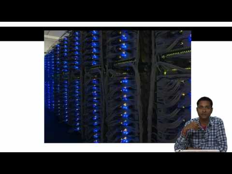
  • So here's, here's a picture.

  • This is what, it looks like inside a data center.

  • So the, the, what you see there is, is the back up racks, and

  • you can see the connections, between, between the racks.

  • Now, once you have such a big cluster,

  • you actually have to do computations on the cluster.

  • Right?

  • And clustered computing comes with its own, challenges.

  • The first and the most major challenge is that nodes can fail.

  • Right?

  • Now a single, node doesn't fail that often.

  • Right? If you,

  • if you just connect, the next node and

  • let it stay up, it can probably stay up for, three years without failing.

  • Three years is about a 1,000 days.

  • So that's, you know, once in a 1,000 days failure isn't such a big deal.

  • But now imagine that you have a 1,000 servers in a cluster.

  • And in your, and if you assume that these, servers fail, independent of each other.

  • You're going to get approximately one failure a day.

  • Which is, still isn't such a big deal.

  • You can probably deal with it.

  • But now imagine something on the scale of Google which has a million servers,

  • in its cluster.

  • So if you have a million servers, you're going to get a 1,000 failures per day.

  • Now a 1,000 failures per day is a lot and

  • you need some kind of infrastructure to deal with that kind of failure rate.

  • Your failures on that scale introduce two kinds of problems.

  • The first problem is that if, you know, if nodes are going to fail and

  • you're going to store your data on these nodes.

  • How do you keep the data and store persistently?

  • What does this mean?

  • Persistence means that once you store the data,

  • you're guaranteed you can read it again.

  • But if the node in which you stored the data fails, then you can't read the data.

  • You might even lose the data.

  • So how do you keep the data stored persistently if like,

  • these nodes can fail.

  • Now the second problem is is is one of availability.

  • So, let's say you're running one of the computations, and this computation is, a,

  • you know, analyzing massive amounts of data.

  • And it's chugging through the computation and

  • it's going, you know, run half way through the computation.

  • And, you know, at this critical point, a couple of nodes fail, right?

  • And that node had data that is necessary for the computation.

  • Now how we deal with this problem.

  • Now in the first place you may have to go back and

  • restart the computation all over again.

  • But if you restart it now and, and, and

  • the computation turns again when the computation is running.

  • So kind of need an infrastructure that can hide these kinds of node failures and

  • let the computation go to go to completion even if nodes fail.

  • The second challenge of cluster computing is that

  • the network itself can become a bottleneck.

  • Now remember, there is this 1 Gbps network bandwidth.

  • That is available between individual nodes in a rack and

  • a smaller bandwidth that's available between individual racks.

  • Though if you have 10 TB of data, and you have to move it

  • across a 1 Gbps network connection, that takes approximately a day.

  • You can do the math and figure that out.

  • You know a complex computation might need to move a lot of data, and

  • that can slow the computation down.

  • So you need a framework that you know, doesn't move data around so

  • much while it's doing computation.

  • The third problem is that distributed programming can be really really hard.

  • Even sophisticated programmers find it hard to write distributed programs

  • correctly and avoid race conditions and various kinds of complications.

  • So here's a simple problem that hides most of the complexity of

  • distributed programming.

  • And, and makes it easy to write you know,

  • algorithms that can mine very massive data sets.

  • So we look at three problems that you know that we face when,

  • when we're dealing with cluster computing.

  • And, Map-Reduce addresses all three of these challenges.

  • Right? First of all,

  • the first problem that we saw was that, was one of persistence and

  • availability of nodes can fade.

  • The Map-Reduce model addresses this problem by storing data redundantly on

  • multiple nodes.

  • The same data is stored on multiple nodes so that even if you lose one of

  • those nodes, the data is still available on another node.

  • The second problem that we saw was one of network bottlenecks.

  • And this happens when you move around data a lot.

  • What the Map-Reduce model does is it moves the computation close to the data.

  • And avoids copying data around the network.

  • And this minimizes the network bottle neck problem.

  • And thirdly, the Map-Reduce model also provides a very

  • simple programming model that hides the complexity of all the online magic.

  • So let's look at each of these pieces in turn.

  • The first piece is the redundant storage infrastructure.

  • Now redundant storage is provided by what's called a distributed file system.

  • Now distributed file system is a file system that stores data you know,

  • across a cluster, but stores each piece of data multiple times.

  • So, the distributed file system provides a global file namespace.

  • It provides redundancy and availability.

  • There are multiple implementations of distributed file systems.

  • Google's GFS is or Google File System, or GFS is one example.

  • Hadoop's HDFS is another example.

  • And these are the two most popular distributed file systems out there.

  • Our typical usage pattern that these distributed file systems are optimized for

  • is huge files.

  • That are in the 100s to, of GB to TB.

  • But the, even though the files are really huge,

  • the data is very rarely updated in place.

  • Right, once, once data is written you know it's, it's very, very often.

  • But when it's updated, it's updated through appends.

  • It's never updated in place.

  • And for example let, let, imagine the Google scenario once again.

  • When Google encounters a new webpage it, it adds the webpage to a depository.

  • Doesn't ever go and

  • update the content of the webpage that it already has crawled, right?

  • So a typical usage pattern consists of writing the data once,

  • reading it multiple times and appending to it occasionally.

  • Lets go into the hood of a distributed file system to see how it actually works.

  • Data is kept in chunks that are spread across machines.

  • So if you take any file, the file is divided into chunks, and

  • these chunks are spread across multiple machines.

  • So the machines themselves are called chunk servers in this context.

  • So here's, here's an example.

  • There are multiple multiple chunks servers.

  • Chunk server 1, 2, 3, and 4.

  • And here's the file 1.

  • And file 1 is divided into six chunks in this case, C0, C1, C2, C3, C4 and C5.

  • And these chunks as you can see four of the chunks happen to be on Chunk server 1.

  • One of them is on Chunks server 2 and, one of them is on Chunks server 3.

  • Now this is not sufficient.

  • You actually have to store multiple copies of each of these chunks and so

  • we replicate these chunks so here copy, here is a copy of C1.

  • On Chunk server 2, a copy of C2 in Chunk server 3, and so on.

  • So each chunk, in this case is replicated twice.

  • And if you notice carefully you'll see that replicas of

  • a chunk are never on the same chunk server.

  • They're always on different chunks of, so

  • C1 has one replica on Chunk server 1 and one on Chunk server 2.

  • C0 has one on Chunk server 1, and one on Chunk server N, and so on.

  • And here is here is another file, D.

  • D has two chunks, D0 and D1.

  • And that's replicated twice.

  • And so and so that's stored on different chunks server [INAUDIBLE].

  • Now so, so you serve you serve from chunk files and

  • store them on, on these, on these chunk servers.

  • Now we turn some of the chunk servers, also act as compute servers.

  • And when, whenever your computation has to access data.

  • That computation is actually scheduled on the chunk server that

  • actually contains the data.

  • This way you avoid moving data to where the computation needs to run,

  • but instead you move the computation to where the data is.

  • And that's how you put a wide under the city data movement in the system.

  • This isn't clear when you look at look at some examples.

  • So the sum of this, each file is split into contiguous chunks.

  • And the chunks are typically 16 to 64 MB in in size.

  • On each chunk is replicated,

  • in our example we saw each chunk replicated twice.

  • But it could be 2x or 3x replication.

  • 3x is the most common.

  • And we saw that the chunks were actually kept on different chunk servers.

  • But, but when you replicate 3x, you know, the system usually makes an effort.

  • To keep at least one replica in a entirely different rack if possible and

  • why do we do that?

  • We do that because it's you know,

  • the most common scenario is that a single node can fail.

  • But it's also possible that the switch on a rack can fail, and

  • when the switch on a rack fails, the entire rack becomes inaccessible.

  • And then if you have all the chunks for a, for in all the replicas of a chunk in

  • one rack then that whole chunk can become inaccessible.

  • So if you keep replicas of a chunk on different racks then even if

  • a switch fails then it can still access that chunk.

  • Right so the system tries to make sure that,

  • that the replicas of a chunk are actually kept on different racks.

  • The second component of a distributed file system is, is a master node.

  • Now the master node is also known as the, it's called a master node in

  • the Google file system, it's a called a Name Node in Hadoop's HDFS.

  • But the master node stores metadata about where the files are stored.

  • And for

  • example, if my you know, it'll know that file one is divided into six chunks.

  • And here is, here are the locations of each of the six chunks, and

  • here are the locations of the replicas.

  • And the master node itself may be replicated because otherwise it

  • might become a single point of failure.

  • The final component of a distributed file system is a client library.

  • Now, when the, when a client, or, or an algorithm that needs to

  • access the data tries to access a file it goes through the client library.

  • The client library talks to the master and

  • finds the chunk servers that actually store the chunks.

  • And once that's done the client is directly connected to the chunk servers.

  • Where it can access the data without going through the master nodes.

  • So the data access actually happens in peer-to-peer fashion without going

  • through the master node

Welcome to Mining Massive Datasets.

Subtitles and vocabulary

Click the word to look it up Click the word to find further inforamtion about it