Placeholder Image

Subtitles section Play video

  • >>

  • So it's my pleasure to introduce to you Geoff Hinton, who is a pioneer in machine learning

  • and neural nets, and more recently [INDISTINCT] architectures. And then, I think that's going

  • to be topic of today. So take it over. >> HINTON: Okay. So I gave it to Okeer a couple

  • of years ago. And the first 10 minutes or so will be an overview of what I said there,

  • and then I'll talk about the new stuff. The new stuff consists of a better learning module.

  • It allows you to learn better in all sorts of different things, like, learning how images

  • transform, learning how people walk, and learning object recognition. So the basic learning

  • module consists of some variables that represent things like pixels, and these will be binary

  • variables for that. Some variables that represent--these are latent variables, they're also going to

  • be binary. And there's a bipartite connectivity, so these guys are connected to each other.

  • And that makes it very easy if I give you the states of the visible variables to infer

  • the states of the hidden variables. They're all independent given the visible variables

  • because it's a non-directed graph. And the input procedure just says, the probability

  • of turning on hidden unit "hj" given this visible vector "v" is the logistic function

  • of the total what he gets from his audience, so very simple for the hidden variables. Given

  • the hidden variables, we can also infer the visible variables very simply. And if we want

  • some--if we put some weights on the connections and we want to know what this model believes,

  • we can just go back and then forward inferring all the hidden variables in parallel than

  • all the visible ones. Do that for a long a time, and then you'll see examples of the

  • kinds of things it likes to believe. And the end of learning is going to be to get it to

  • like to believe the kinds of things that actually happen. So this thing is governed by an energy

  • function that has given the weights on the connections. The energy of a visible plus

  • a hidden vector is the sum overall connections of the weight if both the visible and hidden

  • units are active. So I'm going to pick some of the features that are active, you adding

  • the weight, and if it's a big positive weight, that's low energy, which is good. So, it's

  • a happy network. This has nice derivatives. If you differentiate it with respect to the

  • weights, you get this product of the visible and hidden activity. And so, that the derivative

  • is going to show up a lot in the learning because that derivative is how you change

  • the energy of a combined configuration of visible and hidden units. The probability

  • of a combined configuration, given the energy function, is E to the minus the energy of

  • that combined configuration normalized by the partition function. And if you want to

  • know the probability of a particular visible vector, you have to sum all the hidden vectors

  • that might go with it and that's the probability of visible vector. If you want to change the

  • weights to make this probability higher, you always need to lower the energies of combinations

  • of visible vector on the hidden vector that would like to go with it and raise the energies

  • of all other combinations, so you decrease the computation. The correct maximum likelihood

  • learning rule that is if I want to change the weights so as to increase the log probability,

  • that this network would generate the vector "v" when I let it just sort of fantasize the

  • things it like to believe in is a nice simple form. It's just the difference of two correlations.

  • So even though it depends on all the other weights, it shows up this is difference of

  • correlations. And what you do is you take your data, you activate the hidden units,

  • that's to classify the units, and then we construct, activate, we construct activate.

  • So this is a mark of chain. You run it for a long time, so you forgot where you started.

  • And then you measure the correlation there, start with the correlation here. And what

  • you're really doing is saying, "By changing the weights in proportion to that, I'm lowering

  • the energy of this visible vector with whatever hidden vector it chose. By doing the opposite

  • here, I'm raising the energy, the things I fantasize." And so, what I'm trying to do

  • is believe in the data and not believe in what the model believes in. Eventually, this

  • correlation will be the same as that one. In most case, nothing will happen because

  • it will believe in the data. In terms that you can get a much quicker learning algorithm

  • where you can just go on and [INDISTINCT] again, and you take this difference of correlations.

  • Justifying that is hard but the main justification is it works and it's quick. The reason this

  • module is interesting, the main reason it's interesting is you can stack them up. That

  • is for accompanied reason you're not going to go into it, it works very well to train

  • the module then take that activities of the feature detectors, treat them as so they were

  • data, and train another module on top of that. So the first module is trying to model what's

  • going on in the pixels by using these feature detectors. And the feature detectors would

  • tend to be highly correlated. The second model is trying to model a correlation among feature

  • detectors. And you can guarantee that if you do that right, every time you go up a level,

  • you get a better model of the data. Actually, you can guarantee that the first time you

  • go up a level. For further levels, all you can guarantee is that there's a bound on how

  • good your model of the data is. And every time we add another level, that bound improves

  • if we had it right. Having got this guarantee that something good is happening as we add

  • more levels, we then violate all the conditions of mathematics and just add more levels in

  • sort of [INDISTINCT] way because we know good things are going to happen and then we justify

  • by the fact that good things do happen. This allows us to learn many lesser feature detectors

  • entirely unsupervised just to model instruction of the data. Once we've done that, you can't

  • get that accepted in a machine learning conference because you have to do discrimination to be

  • accepted in a machine learning conference. So once you've done that, you add some decision

  • units to the top and you learn the connections discriminatively between the top-layer features

  • and the decision units, and then if you want you can go back and fine-tune all of the connections

  • using backpropagation. That overcomes the limit of backpropagation which is there's

  • not much information in the label and it can only learn on label data. These things can

  • learn on large amounts of unlabeled data. After they've learned, they you add these

  • units at the top and backpropagate from this small amount of label data, and that's not

  • designing the feature detectors anymore. As you probably know at Google, designing feature

  • detectors is the art of things and you'd like to design feature detectors based on what's

  • in the data, not based on having to produce labeled data. So the edge of backpropagation

  • was design your feature detectors so you're good at getting the right answer. The idea

  • here is design your feature detectors to be good at modeling whatever is going on in the

  • data. Once you've done that, just have a so slightly fine-tune and so you better get right

  • answer. But don't try and use the answer to design feature detectors. And Yoshua Bengio's

  • lab has done lots of work showing that this gives you better minima than just doing backpropagation.

  • And what's more minima in completing different part of the space? So just to summarize this

  • section, I think this is the most important slide in the talk because it says, "What's

  • wrong with million machine learning up to a few years ago." What people in machine learning

  • would try to do is learn the mapping from an image to a label. And now, it would be

  • a fine thing to do if you felt that images and labels are rows in the following way.

  • The stuff and it gives rise to images and then the images give rise to the labels. Given

  • the image, the labels don't depend on the stuff. But you don't really believe that.

  • You only believe that if a label is something like the parity of the pixels in the image.

  • What you really believe is the stuff that gives rise to images and then the labels that

  • goes with images because of the stuff not because of the image. So it's a cow in a field

  • and you say cow. Now, if I just say cow to you, you don't know whether the cow is brown

  • or black, or upright or dead, or far way. If I show an image of the cow, you know all

  • those things. So this is a very high bandwidth path, this is a very low bandwidth path. On

  • the right way to associate labels with images is to first learn to invert this high bandwidth

  • path. And we can currently do that because vision works basically. The first store you

  • look at then, you see things. And it's not like it might be a cow, it might be an elephant,

  • it might be electric theater. Basically, you get it right nearly all the time. And so we

  • can invert that pathway. Having learned to do that, we can then learn what things are

  • called. But you get the concept of a cow not from the name, but from seeing what's going

  • on in the world. And that's what we're doing and then later as I say from the label. Now,

  • I need to do one slight modification to the basic module which is I had binary units as

  • the observables. Now, we want to have linear units with Gaussian noise. So we just change

  • the energy function of it. And the energy now says, "I got a kind of parabolic containment

  • here." Each of these linear visible units has a bias which is like its mean. And it

  • would like to sit here and moving away from that [INDISTINCT] energy. The parabola is

  • the negative log of the Gaussian [INDISTINCT]. And then the input that comes from the hidden

  • units, this is just vi, hj, wij, but Vs have to be scaled by the standard deviation of

  • the Gaussian there. If I ask--if I differentiate that with respect to a visible activity, then

  • what I get is hj, wij divided by the sigma I. And that's like an energy gradient. And

  • what the visible unit does when you reconstruct is it tries to compromise between wanting

  • to sit around here and wanting to satisfy this energy gradient, so it goes to the place

  • where this two gradients [INDISTINCT] opposite and you have--that's the most likely value

  • and then you [INDISTINCT] there. So with that small modification we can now deal with real

  • value data with binary latent variables and we have an efficient learning algorithm that's

  • an approximation of [INDISTINCT]. And so we can apply it to something. So it's a nice

  • speech recognition task that's been well organized by the speech people where there's an old

  • database called TIMIT, it's got a very well-defined task for phone recognition where what you

  • have to do is you're given the short window speech, you have to predict the distribution,

  • the probability for the central frame of the various different phones. Actually, each phone

  • is modeled by 3-state HMMs, sort of beginning middle and end, so you have to predict for

  • each frame is it the beginning middle or end of each with the possible phones, there's

  • a 183 of those things. If you give it a good distribution there to sort of focus on the

  • right thing then all the post-processing will give you back where the phoning bandwidth

  • should be and what your phone arrow radius, and that's all very standard. Some people

  • use tri-phone models. We're using bi-phone models which aren't quite as powerful. So

  • now we can test high goodwill by taking 11 frame of speech. It's 10 milliseconds per

  • frame but each frame is looking at like 25 milliseconds of speech and predicting the

  • phone at the middle frame. We use the standard speech representation which is mel-cepstral

  • coefficients. There's 30 of those, and there are differences and differences and difference,

  • differences; and we feed them in to one of these deep nets so. So here's your input,

  • 11 frames and 39 coefficients. And then--I was away when the student did this and he

  • actually believed what I said. So he thought adding lots and lots of hidden units was a

  • good idea. I've started it too. But he added lots of hidden units all unsupervised, so

  • all this green connections are learned without any use of the labels. He used to bottleneck

  • there, so the number of Reg connections will be relatively small. These are not--these

  • have to be learned using discriminative information. And now you're back propagating the correct

  • answers through this whole net for about a day on a GPU board or a month on a core, and

  • it does very well. That is the best phone error rate we got was 23%. But the important

  • thing is whatever configuration you use, how many hidden layers as long as they are plenty

  • and whatever widths and whether you use this bottleneck or not, it gets between 23% and

  • 24%. So it's very robust to the exact details of how many layers and how wide they are.

  • On the best previous result on TIMIT for things that didn't use speaker adaptation is 24.4%

  • and that was averaging together on lots of models, so this is good.

  • >> So each of these layers that's four million weights?

  • >> HINTON: Yup, four million weights. So we're only training one, two, three, one, two, three,

  • we're training, you know, about 20 million weights. Twenty million weights is about 2%

  • of a cubic millimeter of cortex. I think so, this is a tiny brain. The last, probably,

  • all you need for [INDISTINCT] recognition. >> Why did they start with the differences

  • and double differences of the MFCCs that you're going into a thing that could learn to do

  • that itself if they wanted to? >> HINTON: That's a very good question 'cause

  • you are sitting at the end. It's an extremely good question because the reason I put the

  • differences and double differences is so they can model a data with a diagonal co-variance

  • metric--diagonal co-variance model--and you can't model the fact that overtime two things

  • turn to be very much the same where modeling co-variance is, unless you actually put the

  • differences into the data and you model the differences directly. So it allows you to

  • use a model that conquered with co-variances. Later on we're going to show a model that

  • conquered with co-variances and then we are going to do what the client always said you

  • should do, which is throw away the mel-cepstral representation and use the better representation

  • in speech. >> I said that?

  • >> HINTON: Yes, you said that to me the last time [INDISTINCT].

  • >> Smart guy. >> HINTON: Okay, so the new idea is to use

  • a better kind of module. This module already works pretty well, right? You know, it does

  • well at forming recognition, it does well in all sort of things. It can't model multiplicative

  • interactions very well. It can model anything with enough training data, but its not happy

  • modeling multiplies. It multiplies all over the place. I'll show you a bunch of place

  • where you need multiplies. Here's the sort of main example of why you need multiplies.

  • Supposed I want to, from a high level of description of an object the name of the shape and it's

  • pose, size, position orientation. So, first of all, I want to generate the parts of an

  • object and I want them to be related correctly to each other. I could use very accurately

  • top down model that says none of this square and none pose gram, because I generate each

  • piece in exactly the right position; that would require high bandwidth. Or I could be

  • sloppy and I could say, "I need to generate this side, not sort of a representation and

  • distribution of where this side might be. And I'll generate corners and other sides

  • and they're all a bit sloppy. And if I picked one thing from each distribution, it would

  • make a nice square. But I could also top-down specify how these things should be pieced

  • together. In effect, I can specify a macro form of field; this is what goes with what?

  • And then I can clean this up knowing these distributions and pick a square like that.

  • Of course, I might sometimes pick a square that has slightly different orientation or

  • slightly different size, but it'll be a nice clean square because I know how they go together.

  • And so that's a much more powerful kind of generation model, and that's what we want

  • to learn to do, and so we are going to need hidden units up here to specify interactions

  • between visible units here, as opposed to just specifying input of visible units. There's

  • an analogy for this, which is, if I'm an officer and there's a bunch of soldiers and I want

  • them to stand in the square, I could get out my GPS and I can say, "Soldier number one,

  • stand at this GPS coordinates. And soldier number two, stand at these GPS coordinates."

  • Now, if I use enough digits, I'll get a nice neat rectangle, or I could say, "Soldier number

  • one, stand roughly around here. And then soldier number two, hold your arm out and stand this

  • distance from soldier number one." And that's a much better way to get a neat rectangle.

  • It will cause far less communication. So what you're doing is you're downloading roughly

  • where people should stand and then how they should relate to each other. We have to specify

  • the relations not just where they should be. And that's what we'd like in a powerful [INDISTINCT]

  • model. So, we're going to aim to get units in one layer to say how units in the layer

  • below should latterly interact when you generate it. It's going to turn out you don't need

  • to worry about these lateral interactions when you recognize it. When you generate,

  • you do. To do that, we're going to need things called third-order Boltzmann machines, which

  • has three lane tractions. So Terry Sejnowski, he pointed out a long time ago that we have

  • an energy function like this where this was V and this was H, but these are just binary

  • variables. And we could probably well write down an energy function like this with three

  • things in tract, then we have a three layer weight. And if you think about these three

  • things now, K, the state of K is acting like a switch. When K is on, you effectively have

  • this weight between I and J. When K is off, this weight disappears. And it happens every

  • which way because it's symmetric. So using an energy function like this, we can allow

  • one thing to specify how two other things should interact. So each hidden unit can specify

  • a whole mark of random field over the pixels if you want. But that sort of begins to make

  • you worry because a mark of random field has a lot of parameters in it. And if you start

  • counting in the sits here, if you have any of these and any of those and none of those,

  • you get enqueued to these parameters which is rather a lot. If you're willing to use

  • enqueued parameters, you can now make networks to look like this. Suppose I have two images

  • and I want to model how images transform over time, unless suppose I'm just moving random

  • dots around, have a pan of random dots and I translate it. Well, if I see that dot and

  • I see that dot, that's some evidence for a particular translation. And so if I put a

  • big positive weight there, this triangle is meant to interrupt that big three-way weight.

  • Then when this and this around, they'll say it's very good to have this guy up. It would

  • have been nice at low energy state. If I also see this pair of dots, I'll get more routes,

  • though, and this guy should be--and I will turn this guy on. If however this pixel went

  • to here, I'll go for this guy. And if this pixel also went to there but this guy--so

  • these guys are going to represent coherent translations of the image, and it's going

  • to be able to use these three-way weights to take two images and extract two units that

  • represent the coherent translation. It'll also be able to take the pre-image and the

  • translation, and compute with pixel should be on here. Now what we're going to do is

  • take that basic model and we're going to factorize it. We're going to say, "I've got these three-way

  • weights and I've got too many of them." So, I'm going to represent each three-way weight

  • as the product of three two-way things. I'm going to introduce these factors and each

  • factor is going to have these many parameters which is just pro-factor, is just a linear

  • number of parameters. If I have about N factors, I end up with only N square of these weights.

  • And if you think about how pixels transform in a new image, they don't do random permutations.

  • It's not that this pixel goes on that one, goes here. Pixels do sort of consistent things,

  • so I don't really need enqueued parameters because I'm just trying to model these fairly

  • consistent transformations, which is a limited number, and I should be able, too, in many

  • less parameters. And this is the way to do it. So, that's going to be our new energy

  • function given the bias terms. One way of thinking about how modeling a weight is I

  • want these tensor of three-way weights. If I take an IF product and two vectors like

  • this, I'll get a matrix that has rank one. So I get a three-way product. I'll get a tensor

  • that has rank one. And if I now add up a bunch of tensors like that so each factor now, each

  • F, specifies a rank one tensor, by adding up a bunch of them, I can model any tensor

  • I like if I use N square factors. If I use any N factors, I can model most regular tensors

  • but I can't model arbitrary permutations, and that's what we want. If you ask how does

  • inference works now, inference is still very simple in this model. So here's a factor.

  • Here's the weights connecting it to, say, the pre-image. Here's the weights connecting

  • it to the post-image. Here's the weights connecting it to the hidden units. And to do inference

  • what I do is this. Supposed I only have that one factor. I would multiply the pixels by

  • these weights; add all that up so I get a sum of this vertex. I do the same here; I

  • get a sum of this vertex. Then I multiply these two sums together to get a message going

  • in the center of the hidden units. And as that message goes to the hidden unit, I multiply

  • it by the weight on my connection. And so what the hidden unit will see is this weight,

  • turns the product of these two sums, and that is the derivative of the energy with respect

  • to the state of this hidden unit, which is what it needs to know to decide whether to

  • be on or off, it wants to go into what other state below the image. And all the hidden

  • units remain independent even though I've got these multipliers now. So this is much

  • better than putting in another stochastic binary unit here. If I put a stochastic binary

  • unit in here, the hidden units would cease to be independent and inference will get tough.

  • But this way, whether a deterministic factor that's taking a part of these two sums, inference

  • remains easy. The learning also remains easy. So this is the message that goes from factor

  • F to hidden unit H, and that message is the product that we got of these two lower vertices;

  • the product of the sums, the compute on the pre-image and the post-image. And the way

  • you learn the weight on the connection from factor F to hidden unit H is by changing the

  • weight so as to lower the energy when you're looking at data, and raise the energy when

  • you're constructing these from the model or just reconstructing things from the hidden

  • units you got from data. And those energy groups, they just look like this. They're

  • just the product of the state of the hidden unit and the message that goes to it when

  • you're looking at data and the state of the hidden unit and the message that goes through

  • it when you're looking at samples from the model or reconstructions. So it's still a

  • nice pair-wise learning rule. So everything is pair-wise still, so you might fit into

  • the brain. Now, if we look what one of these factors does when I show random dot patterns

  • to translate, then we can look at the weights connecting it to the pre-image, and that's

  • a pattern of weights where white is a big positive weight, black is a big negative weight

  • because that would have a learned a great in connecting it to the pre-image and this

  • will have learned a great in connecting it to the post-image. With a hundred factors,

  • I'll show you what Roland learned. So, those are the hundred the hundred factors connecting--these

  • are the receptive fields at the factors in the pre-image. And remember it's looking at

  • translating dots, and these are the factors in the post-image. And you see, it's basically

  • learned the freer basis and it's learned to translate things by about 90 degrees. And

  • that's a very good way of handling translation. Mathematicians say things like, "The freer

  • basis is a natural basis for modeling translation." I don't really know what that means, but just

  • learn the freer basis on that. And if you get rotations, it learned the different basis.

  • So this is the basis that learns for rotations. You see it learns about yin and yang here.

  • Oops [INDISTINCT]. Okay, that's the basis for rotations. One other thing you could do

  • is train it just on single dot pans and translating in a coherent way and then test it on two

  • overlaid dot patterns but they're translating different directions. It's never seen that

  • before. It's only been trained on coherent motion where we're going to test it on what's

  • called transparent motion. In order to see what it thinks, when we train the uncivilized,

  • there's no labels anywhere, we never tell it what the notions are, we need some way

  • to seeing what it's thinking, so we add a second hidden layer that looks at the hidden

  • units representing transformations and it's fairly sparse. So the units on that second

  • hidden layer will be tuned to particular directions of motion. And then to see what it's thinking,

  • we take the directions those units like weighted by how active those units are and I will tell

  • you what directions it thinks it's seeing. Now when you show it transparent motion and

  • you look at those units in the second hidden layer, if the two motions are within about

  • 30 degrees, it sees a single motion of the average direction. If they're beyond about

  • 30 degrees, it sees two different motions and once more they're repelled from each other.

  • That's exactly when I was with people, and so this is exactly how the brain works. Okay.

  • There's going to be a lot of that kind of reasoning in this talk. I'm going to on to

  • time series models now. So, we'd like to model not just static images, for example, we like

  • to model video. To be [INDISTINCT] we're going to try something a bit simpler. When people

  • do time series models, you would nearly always like to have a distributed non-linear representation,

  • but that's hard to learn. So people tend to do dumb things like Hidden Mark up Models

  • or Linear Dynamical Systems which either give up on the distributed or on the non-linear,

  • but are easy to doing inference. What we're going to come up with is something that has

  • the distributed and the non-linear and is easy to do inference, but the linear algorithm

  • isn't quite right but it's good enough. It's just an approximation to make some [INDISTINCT].

  • And the inference also is ignoring the future and just basing things on the past. So, here's

  • a basic module, and this is with just two-way interactions. This is the Restricted Boltzmann

  • Machine with visible units and hidden units. Here are the previous visible frames. These

  • are all going to be linear units. And so, these blue connections are conditioning the

  • current visible values on previous observed values in a linear way. So, it's called an

  • autoregressive model. The hidden units here are going to be binary hidden units; they're

  • also conditioned on previous visible frames, and learning is easy in this model. What you

  • do is you take your observed data, and then given the current visible frame and given

  • the previous visible frames, you got import to the hidden units, they're all independent

  • given the data, so you can separately decide what states they should be in. Once you fixed

  • states for them, you now reconstruct the current frame using the input you're getting from

  • previous frames and using the top you got in from the hidden units. After we construct,

  • you then activate the hidden units again. When you say the difference in the power statistics

  • with data here and the reconstructions here to learn these weights and you take the difference

  • on activities of these guys with data with reconstructions to get signal that you can

  • used to learn these weights or these weights. So learning is straightforward and it just

  • depends on differences, and you can learn a model like this. After you've learned it,

  • you can generate from the model by taking some previous frames. These inputs, the conditioning

  • inputs, in effect, fixed the biases of these to depend on the previous frames. So, these

  • are the dynamic biases, and with these biases fixed, you just get backwards and forwards

  • for awhile and then pick a frame there, and that's your next frame you regenerated, then

  • you keep going. So, we can generate from the model once it learns so we can see what it

  • believes. >> You always go back two steps in time or

  • is that just an example? >> HINTON: Sorry.

  • >> Oh, you were just going back only two steps in time?

  • >> HINTON: No, we're going to get back more sets in time.

  • >> Okay, and you let... >> HINTON: I just got lazy with the PowerPoint.

  • Now, one direction we could go from here is to higher level models. That is, having learned

  • this model where these hidden units are all independent given the data, we could say--well,

  • what I've done is I've turned the visible frames into the hidden frames map. And it

  • turns out you can get a better model if you take these hidden frames, a model what's going

  • here, and now you put in conditioning connections between the hidden frames and more hidden

  • units that don't have conditioning here that don't interact with other hidden unit. [INDISTINCT]

  • in this model. Then you can prove that if you do this right, then you'll get a better

  • model of the original sequences or your improver band on the model of the original sequences.

  • So you can [INDISTINCT] lots of layers like that. And when you have more layers, it generates

  • better. But I'm going to go in a different direction. I'm going to show you how to do

  • it with three-way connections. And we're going to apply it to motion-capture data, so you

  • put reflective markers on the joints, you have lots of infrared cameras, you figure

  • out where the joints are in space. You know the shape of the body so you go backwards

  • through that to figure out the joint angles and then the frame of data is going to consist

  • of 50 numbers, about 50 numbers which are joint angles and the translations and rotations

  • of the base of the spine. Okay. So, imagine we got--one of these mannequins you see in

  • art shop windows, we got a pins stuck in the base of his spine and we can move him around

  • and rotate him using this pin and we can also wiggle his legs and arms. Okay. And what we

  • want him to do is as we move him around, we want him to wiggle his legs and arms so his

  • foot appears to be stationary on the ground and he appears to be walking. And he'd better

  • wiggle his leg just right as we translate his pelvis, otherwise his foot will appear

  • to skid on the ground. And we're going to model him, we can do hierarchal model like

  • I just showed you or we can a three-way model like this where we condition six earlier of

  • frames, this is a current visible frame, here's basic bolts in the machine accept that it's

  • neither one of these 3-way things where these are factors. And we have a 1-of-N style variable.

  • So, we have data and we tell it the style when we're training it, so that's sort of

  • semi-supervise. It learns to convert that 1-of-N representation in to a bunch of real

  • value features and then it uses this real value features as one of the inputs to a factor.

  • And what the factor are really doing is saying, these real value features are modulating the

  • weight matrixes that use for conditioning and also this weight matrix that use in your

  • parallel linear model. So, these are modulating an auto aggressive model. That's very different

  • from switching between auto aggressive model it's much more powerful. Yeah?

  • >> I missed with what this one event is...? >> HINTON: So, we're going to have data of

  • someone walking in various different styles. >> Styles of walking.

  • >> HINTON: The style of walking. Yeah. >> So you mean your earlier diagram when you

  • can't beat history, it looked like there was nothing to keep track in the relative order

  • of the earlier direct delta direct link because... >> HINTON: Yes.

  • >> ... is there anything in the model that cares about that relative...?

  • >> HINTON: Yeah. Yeah. The weights on the connections will tell you which frame it's

  • coming from. Right. In the earlier model, there were two blue lines, they're different

  • matrixes and they have different weights on. >> There's nothing from two steps to previews

  • to ones step previews, right, it just skip all the way?

  • >> HINTON: It just skipped all the way, right. You just...

  • >> Will that continue to happen? >> HINTON: Yes. In other words there's direct

  • connections from all six previous frames to the current frame for determining the current

  • frame. >> Right. And then what links from the six

  • frames of the fifth earliest report? >> HINTON: Well, there where when you were

  • computing what the fifth frame was doing, right?

  • >> Okay. >> HINTON: But when we're computing this frame

  • we have direct connections from it. Okay. So, we're now going to train this model, it's

  • relatively easy to train especially on the GPU board, and then we're going to generate

  • from it, so we can see sort of what it learned and we can judge if it's doing well by whether

  • the feet slip on the ground. All right. >> [INDISTINCT]

  • >> HINTON: We'll get there. >> Sorry.

  • >> HINTON: Here's a normal walk. Maybe, at least they're willing. Okay. So I was generating

  • from the model--he's deciding which direction to turn in, and he's deciding, you know, he

  • needs to make the outside leg go farther than the inside leg and so on. If we--we have one

  • model but if we flip the style label to say, gangly teenager, he definitely looks awkward.

  • Right. We've all been there. I think this is a computer science student. My main reason

  • for thinking that is if you asked him do a graceful walk, it looks like this. And that's

  • definitely C3PO. >> [INDISTINCT].

  • >> HINTON: Now, I think this was a student [INDISTINCT]--but he's very good. You can

  • ask him to walk softly like a cat. We're asking to model at present, right? The model looks

  • pretty much like the real data the real data obviously the feet are planted better but

  • notice, he can slow down then speed up again. Auto aggressive models can't do things like

  • that, Auto aggressive models have a biggest size in value, the size is bigger than one

  • in which case they explode or a smaller one in which case they die and the way to keep

  • them alive is by keep--you keep injecting random noise so that they stay alive and that's

  • like making a horse walk by taking a dead horse and jiggling it, it's kind of--it's

  • not good. Now, he doesn't have any model of the physics so, in order to do this kinds

  • of stumbles, there had to be stumble similar to that in the data but when he stop in which

  • he stumble he did when, he's entirely determining. We could make him do a sexy walk but you're

  • probably not interested in that. >> I just order a chicken.

  • >> HINTON: You want dinosaur the chicken? Where's dinosaur the chicken?

  • >> And chicken, number five. >> At number five.

  • >> HINTON: Oh, no, that's dinosaur and chicken. That's a blend. Maybe a switch. He's got quite a lot of foot

  • [INDISTINCT] that's probably a blend. This is doing a sexy walk and then you flip the

  • label to normal and then you flip it back to sexy. It's never seen any transitions but

  • because all one model, it can do reasonable for transitions.

  • >> So you have these hundred style variables, can you de-couple those form the one event

  • style and just make up new styles by playing with those...

  • >> HINTON: Yup. Yup. Now, you can also give it many more labels when you train, you can

  • give it speed, stride length all sorts of things then you can control it very well,

  • yeah. Okay. So, you can learn time series at least for 50 dimensional data and obviously

  • what we all want to do is apply that to video but we haven't done that yet. Except for some

  • very simple cases. The last thing I'm going to show is the most complicated use of these

  • 3-way models. One way of thinking of it, so that it's similar to the previous uses, is

  • that we take an image and we make two copies of it but they have to be same. And then we

  • insist the weights that go from a factor of this copy are the same as the weights that

  • go from the factor of this copy. So if I=J, WI=WJF. Inference is still easy in fact inference

  • here will consist of--you take these pixels times these weights to get a weighted sum,

  • and then you square it because this is going to be the same weighted sum. So, inference

  • consist--take linear filter, square its output, and send it by these weights to the hidden

  • units. That's exactly the model called the [INDISTINCT] energy model, is right, kind

  • of linear filter. This is being proposed both by Vision people by Adelson and Bergen, a

  • long time ago in the '80s, and by neuroscientists. So, neuroscientists had tried to take simple

  • cells, my point vaguely about, and look at what polynomial they're output is of their

  • input, and Yang Dan at Berkeley says it's between 1.7 and 2.3, and that's means two.

  • So, this looks quite like models that were proposed for quite different reasons and it

  • just drops out of taking a 3-way imaging model and factorizing it. The advantage we have

  • is that we have a learning algorithm for all these weighs now, when we generative model.

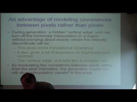
  • So now we can model covariances between pixels, and the reason that's good is–-well, here's

  • one reason why it's good. Suppose I asked you to define a vertical edge. Most people

  • will say, "Well, vertical edge is something that light on the side and dark on that side.

  • Well no, maybe it's light on this side and dark on that side, but you know. Well, it

  • could be light up here and dark down there, and dark up here and light down there." Okay.

  • Or it could be texture edge. It's getting--oh, it might actually be a disparity edge. Well,

  • the manner should be motion this side and no motion that side. That's a vertical edge

  • too. So, a vertical edge is a big assortment of things, and what all those things have

  • in common is vertical edge is something where you shouldn't do horizontal interpolation.

  • Generally new image, horizontal interpolation works really well. A pixel is the average

  • of its right and left neighbors, pretty accurately almost all the time. Occasionally it breakdowns,

  • and the place it breaks down is where there is a vertical edge. So, a real abstract definition

  • of vertical edge is breakdown of horizontal interpolation. And that's what our models

  • are going to do. A hidden unit is going to be putting in interpolation, and it's actually

  • going to turn-off sort of reverse logic, when that breaks down its going to turn-off, so

  • one way of seeing it is this. If this hidden unit here is on, it puts in a weigh between

  • pixel I and pixel J that's equal to this weight times this weight, times this weight. Okay.

  • Since theseokay, that's good enough. So, these are controlling affectively the mark

  • of random field between the pixels, so we can model covariances nicely. Because the

  • hidden units are creating correlations between the visible units reconstruction is now more

  • difficult. We could reconstruct one image given the other image, like we did with motion,

  • but if you want to reconstruct them both and make them identical it gets to be harder.

  • So, we have to use a different mathical Hybrid Monte Carlo. Essentially you start where the

  • data was and let it wonder away from where it was but keeping both images the same. And

  • I'm not going to go to Hybrid Monte Carlo, but it works just fine for doing the learning.

  • And the Hybrid Monte Carlo is used just to get the reconstructions and the learning algorithm

  • just the same as before. And what we're going to do is we're going to have some hidden units

  • that are using these 3-way interactions to model covariances between pixels, and other

  • hidden units are just modeling the means. And so we call-–for meaning covariance,

  • we call this mcRBM. Here's an example of what happens after it's learned on black and white

  • images. Here's an image patch. Here's its reconstruction of the image patch, if you

  • don't have noise, which is very good, from the mean and covariance units. Here's the

  • stochastic reconstruction which is also pretty good. But now we're going to do something

  • funny, we're going to take the activations of the covariance units. The things that are

  • modeling which pixels are the same with which other pixels and we're going to keep those.

  • But we are going to take the activations of the mean units, so we're going to throw those

  • away, and pretend that the means from the pixels look like this. Well, let's take this

  • one first. We tell all the pixels have the same value, except these are which are much

  • darker and it now tries to make that information about means fit in with these information

  • about covariances which is of these guys should be the same but very different from these

  • guys. And so, it comes up with the reconstruction that it looks like that. Where you see it's

  • taken this dark stuff and blurred across this region here. If we just give it four dots

  • like that, and the covariance matrix you've got from there, it'll blur those dots out

  • to make an image that looks quite like that one. So this is very like what's called the,

  • kind of watercolor model of images, where you know about where the boundaries are and

  • you just, sort of, roughly sketching the colors of the regions and it all looks fine to us,

  • because we sort of slaved the color boundaries to the actual--where the edges are. If you

  • reversed the colors of these it produce the reversed image because the covariance doesn't

  • care at all about the signs of things. If you look at the filters at your lens, the

  • mean units which are for sort of coloring in regions, learn these blurry filters--and

  • by taking some combination of a few dozen of those you can make more or less of what

  • other colors you like anywhere. So, very blur there-–smooth, blurry, and multicolored

  • and you can make roughly the right colors. The covariance units learn something completely

  • different. So, these are what the filters learned and you'll see that, those factors,

  • they learn high frequency black and white edges. And then a small number of them, turning

  • to low frequency color edges that are either red, green, or yellow blue and what's more

  • when you make it from a topographic map using a technique I'll describe on the next slide.

  • You get this color blob, this low frequency color blob in with the low frequency black

  • and white filters. And that's just what you see in a monkey's brain, pretty much. If you

  • go into a monkey's brain you'll see these high frequency filters whose orientation changes

  • smoothly as you go through the cortex tangentially, and you'll see these low frequency color blobs.

  • Most neuroscientists thought that at least must be innate. What this is saying is, "Nope.

  • Just the structure of images is, and the idea of forming a topographic map, is enough to

  • get this." That doesn't mean it's not innate, it just means it doesn't need to be. So the

  • way we get the topographic map is by this global connectivity from the pixels to the

  • factors. So the factors really are learning local filters. And the local filters start

  • off colored and gradually learn to be exactly black and white. Then there's local connectivity

  • between the factors in the hidden units. So one of these hidden units will connect to

  • a little square of factors and that induces a topography here and the energy function

  • is such that when you turn off one of these hidden units to say smoothness no longer applies,

  • you pay a penalty. And you derive to just pay the penalty once. And so two factors is

  • going to come on at the same time, it's best to connect them to the same hidden unit so

  • you only pay the penalty once. And so that will cause similar factors to go to similar

  • places in here when we get a topographic map. For people who know about modeling images,

  • as far as I know, nobody has yet produced a good model of patches of color images. That

  • is the genres of model that generates stuff that looks like the real data. So, here's

  • a model that was learned on 16x16 color images from the Berkeley database and here's these

  • generated from the model. And they look pretty similar. Now, it's a partly a trick, the color

  • balance here is like the color balance and it makes you think they are similar. But,

  • it's partly real. I mean, most of these are smooth patches of roughly uniform color as

  • are most of these. These are few more of these as smooth than those. But you also get these

  • things where you get fairly sharp edges, so you get smoothness than a sharp edge than

  • more smoothness, like you do in the real data. You even get things like corners here. We're

  • not quite there yet but this is the best model there is in patches of color images. And it's

  • because it's modeling both the covariance and the means, so it's capable of saying,

  • "What's the same as what?" As well as, "What the intensities are?" You can apply it for

  • doing recognition. So this is a difficult object recognition to ask where this 80 million

  • unlabelled training images; not only of these classes but of thousands and thousand of classes.

  • They were collected by people at MIT. It's called the Tiny Images database. They're 32x32

  • color images. But it's surprising what you can see in a 32x32 color image. And since

  • the biggest model we're going to use has about a hundred million connections, that's about

  • 0.1 of a cubic in ratio of cortex in terms of the number of parameters, and so we have

  • to somehow give our computer model some way of keeping up with the brain which has a lot

  • more hub, right? And so we do it by giving it a very small retina. We say, "Suppose the

  • input was only 32x32, maybe we can actually do something reasonable there." So as you'll

  • see there are a lot of variations. If you look birds, that's a close up of an ostrich,

  • this is a much more typical picture of a bird. And it's hard to tell the difference within

  • these tiny categories. Particularly things like deer and horse. We deliberately chose

  • some very similar categories like truck and car, deer and horse. People are pretty good

  • at these. People won't make very many errors. That's partly because these were hand-labeled

  • by people, so. But even people make some of errors. We only have 50,000 training examples.

  • Five thousand of each class and ten thousand test examples, because we have to hand-label

  • them, but we have a lot of untrained--unlabelled data. So we can do all these pre-training

  • on lots of unlabelled data and then take out covariance units on our mean units and just

  • try doing multi-[INDISTINCT] on top of those, or maybe add another hidden layer and do it

  • on top of that. So, what Marc'Aurelio Ranzato actually did since he worked in Yann LeCun's

  • lab, he actually took smaller patches learned the model and then strode them across the

  • image and replicated them. So it's a sort of a semi-convolutional. And then took the

  • hidden units of all of these little patches and just concatenated them to make a great

  • big vector of 11,000 hidden units which are both the means on the covariances. And then

  • we're going to use that as our features and see how well we can do. And we're going to

  • compare it with various other methods. So the sort of first comparison, you just take

  • the pixels and do logistic ration on the pixels to slide on the tiny glasses. You get 36%

  • right. If you take GIST features which has developed by Torralba and the people at MIT,

  • which were meant to capture what's going on under the image quite well, but they're fairly

  • low dimensional, you get 54%. So they're much better than pixels. If you take a normal RBM

  • which has linear units with glass and noises input variables and then binary hidden units,

  • and then you use those binary hidden units to do castigation, you get 60%. If you use

  • one of these RBMs with both the units like these once for doing the means, and then these

  • units with the three range interaction for modeling covariances, you got 69%; as long

  • as you use a lot of these factors. And if you then learn an extra hidden layer of 8,000

  • units--so now it's just that times that is a hundred million, so there's an extra hundred

  • million connections you learn there. But that's fine because it's unsupervised then you just

  • learn it on lots of data. You get up to 72%. And that's the best result so far on this

  • database. One final thing, you can take this model that was develop for image patches and

  • the student that'll be doing framing recognition just took that code and applied it to log

  • spectrograms, which is sort of more close to what they would like to see, you're not

  • using all these mark up fool stuff, which is designed to throw away stuff you think

  • you don't need and get rid of lots of correlations. Instead you're going to take data that has

  • lots of correlations in but we got a model that can deal with that stuff now. And the

  • first thing George tried on February the 20th, which was four layers of a thousand hidden

  • units on top of this, he got 22.7 correct--percent correct; which was the record for phoneme

  • recognition on the TIMIT database where your not trying to do a model adapted to each speaker.

  • And then a week later when he did that to TIMIT and use more frames, he was down to

  • 21.6%. So this--all this stuff was designed to do vision. It wasn't designed to do phonemes.

  • And if we treat phoneme recognition, it's just a vision problem on a lot of spectral

  • ground. We can wipe out the speech class, at least on small vocabulary. Another student

  • is now, at Microsoft, is seeing if this will work on big recovery as well.

  • >> [INDISTINCT] >> HINTONS: Yes. Yes, right.

  • >> We can give them new better tools. >> HINTONS: We can give them new and better

  • tools. So here's phoneme recognition over the years. Backprop from the 80's got 26.1

  • percent correct. Over the next 20 years or so, they got that down to 24.4 percent, using

  • methods that weren't learning-inspired so we'll call them artificial. We then got down

  • to 21.6 percent; an estimate of human performance is about 15 percent. I don't know much about

  • how they did this estimate, I'm afraid. But we're about--we're nearly a third of the way

  • from artificial TIMIT. And so we need two more ideas and we're there. Okay, I'm done.

  • I'm finished. >> Questions?

  • >> HINTONS: Yes? >> You mentioned YouTube recently announced

  • that the [INDISTINCT] have broken the world record on the end list of data sets of phoneme

  • recognition by simply using a seven layered feed forward network trained with backprop,

  • but doing it on a GPU with lots and lots of cycles.

  • >> HINTONS: Yes, he did indeed announce that. What he didn't announce was--he's got a spectacular

  • result. He gets timed to 35 errors. What he didn't announce was there's two tricks involved.

  • One trick is to use a big net with lot of layers in a GPU board. That trick by itself

  • wouldn't give you 35 errors. There's a second trick which was sort of pioneered by people

  • at Microsoft in fact, which is to put a lots of work into producing distortions of the

  • data so you have lots and lots of labeled data. So you take a labeled image of a two

  • and you distort it in clever ways and make it still look like a two but be translated

  • so people can then get down to about 40 errors. >> I think they patented that already.

  • >> HINTONS: Good. So Dick's already patented that. So you get down to--you can get down

  • to by 40 errors by doing these distortions. What he did was even better distortions, or

  • more of them, and a much bigger net on a GPU and he got from a 40 to 35, which is impressive

  • because it is hard to make any progress there. But it won't work unless you have a lot of

  • labeled data. And what's--the disguised thing is the work went into--if you look in the

  • paper, it's always straightforward, its just backprop, except when you get to the section

  • of how they generated all those sector labeled data where there's very careful things, like

  • if it's a one or a seven they'd only rotate it a certain number of degrees but if it's

  • something else they rotate it in more degrees. I'm actually the referee for this paper but

  • I don't mind him knowing. I think it's a very important work. But he should emphasize that

  • they have to have labeled data to do that, and they have to put work into distortions.

  • So for me the lesson of that paper is when we small computers, you should put your effort

  • into things like weight constraints so you don't have too many parameters because you

  • only got a small computer. As computer gets bigger and faster, you can transfer your effort

  • from, instead of tying the weights together, like Yann was doing in the early days, put

  • your effort into generating more distortions so you can inject your prior knowledge in

  • the form of distortions and that's much less complication-efficient over the big computers,

  • it's fine and it's more flexible. So I think that's the lesson of that paper.

  • >> I shouldn't even need to ask you a question, you answered it. Thank you.

  • >> HINTON: Any other long question? >> It seems like you've invented some kind

  • of a cortex here that house you expect the property that if it does vision it'll do sound.

  • >> HINTONS: Yes. >> What other problems you going to apply

  • it to? >> HINTONS: Maybe it'd be quicker to say the

  • problems we're not going apply. >> Okay.

  • >> HINTONS: I can't think of any. I mean--okay, let me say what the main limitation of this

  • is for vision. We got at least 10 billion neurons for doing visual things; or at least

  • a billion anyway, probably, 10 billion. And even if we got that many neurons and about

  • 10 to the 13 connections for doing vision, we still have a retina that's got a very small

  • phoneme the size of my thumb there at arms length. And so we still take almost everything

  • and don't look at it. I mean, the essence of vision is not to look at almost everything

  • intelligently; and that's why you got all this funny illusions where you don't see things.

  • We have to do that in these models. These models are completely crazy. And all of computer

  • visions are completely crazy, almost all of it. Because they take a uniform resolution

  • image, and quite a big one like a thousand by thousand, and they try and deal with it

  • all at once with filters all over the image. And if they going to do a selection, they

  • either do it by running off their face to get to everywhere, with no intelligence, or

  • they do sort of interest point detection at a very low level to decide what to attend

  • to. What we do is we fixate somewhere. Then on the basis of what our retina gives us,

  • with these big pixels around the edges and small pixels in the middle, we sort of decide

  • what we seeing and where to look next and by the second or third fixation we've fixating

  • very intelligently and the essence of it is that vision is sampling, it's not processing

  • everything; and that's completely missing from what I said. Now in order to do that,

  • you have to be able to do take what you saw and where you saw it and combined them and

  • that will multiply. So this module, it can do multiply. It's very good in combining what's

  • and where's, to integrate information at a time. And that's one of the things, we're

  • working on that. But that's probably the biggest thing missing. But that is an example of having

  • a module is quite good but now it's never good enough, so you have to put it together

  • over time and use it many times. And that's what sequential reasoning in all this stuff

  • are. So basically, as soon people become sequential we're not modeling that at all. We're modeling

  • what you can do in hundred milliseconds. And so that's what's missing. But I believe that

  • to model that sequential stuff we need to understand what is the sequence of, is the

  • sequence of these very powerful operations. And we're in a better shape now to try and

  • model sequential AI, than we were if we didn't know what a primitive operation is. So this

  • sort of primitive operation was just deciding whether two symbols are the same. We're going

  • to be out of luck for understanding how people do sequential stuff. Yeah.

  • >> This is a [INDISTINCT] question as he said he wanted to do everything if it connects.

  • Are you going to do [INDISTINCT] logic like there exists a God and every girl has a boy

  • she loves? >> HINTON: Hang on, I'm still processing that.

  • Right. Right, I'm making the point that people find "quantifies" quite difficult.

  • >> Oh, yeah. If you [INDISTINCT] quantifiers... >> HINTON: I would love to do that. I have

  • not got a clue how to do it. And you will notice that in old-fashioned AI that you used

  • to point out to [INDISTINCT] people, then you can't do quantifiers, so forget it. Nowadays,

  • when they all do graphical models, they didn't mention that anymore because the graphical

  • models have difficulty of it too. Some people has got [INDISTINCT] some people do. Right.

  • Yeah, some people do. But most of the graphical models of, like, five years ago, they do quantifiers

  • either. And so, a pretty good division line would be what you can do without having to

  • deal with really sophisticated problems like that. I would love to know how we deal with

  • that, but I don't. >> Thank you.

  • >> HINTON: So, yeah, I'm going to give up on that right now.

  • >> So if you had 80 million labeled images and no extra unlabeled ones, would you do

  • your pre-training... >> HINTON: Yes. Yes

  • >> ...and then fine tuning to make us better? >> HINTON: In TIMIT, that's what we have.

  • In TIMIT, all the examples we have labels. It stirs a big wind to do the pre-training.

  • >> But you didn't sneak this result I'm just hearing about? It seems to suggest...

  • >> HINTON: Well, the audience switched it but I haven't tried with all these distortions

  • during pre-training. Now, I've assumed student called [INDISTINCT] who just produced a thesis.

  • Well, he tries things like that. He tries distortions in earnest and he uses special

  • distortions of his own. And the fact is distortions helped a lot. But if you do pre-training,

  • that helps some more too. And [INDISTINCT] results, yes, [INDISTINCT] results, suggest

  • that pre-training will get you through different part of the space even if you have all these

  • labeled data. So clearly, one thing that needs to be done is to try the pre-training and

  • combine with these labels. You don't have to have the pre-training, but I bet you, it

  • still helps. And I bet you, it's more efficient too. It's faster because the pre-training

  • is rather pretty fast, you always have to learn a very good model. You got lots of its

  • features. And starting from there, I think, you'll do better than he does just started

  • from random, and faster. That's just a prediction. You might even get done to 34 out of this.

  • The problem with [INDISTINCT] you can't get significance. TIMIT is really nice that way.

  • They designed it well, so you get higher rates. So you can see differences.

  • >> On the time series aspect, did you see anything that would you get inferences or

  • alterations that are beyond the size of the time window you're using?

  • >> HINTON: Sorry, I didn't understand the question. We have a limited time. We don't...

  • >> You have limited time, after training is there anything of a model that picks up...

  • >> HINTON: Nothing. >> Nothing.

  • >> HINTON: Nothing. It cannot deal with--it can't model host...

  • >> It has an internal state. It has an internal state.

  • >> HINTON: Right. But if sort of what happened 15 times steps ago really tells you what should

  • happen now, and it only tells you what you should happen now. It doesn't tell you what

  • should happen in TIMIT 14 times steps. It just contains information across 15 times

  • steps without having a signature of smaller time scales. You can't pick up on that.

  • >> Okay. >> HINTON: Because it's not got a hidden forward-backward

  • algorithm. A forward-backward algorithm potentially could pick up a lot of load, actually can't.

  • >> So this one wouldn't pick up on things like object permanence or all rules behind

  • the box and comes out of the other side and they're not going to be able to...

  • >> HINTON: Not over a long time scale, no, no. Unless you say that there's a memory involved

  • when you go back to a previous--it gets more complicated, right? Now, it is true that when

  • you build the multilevel one, which you can do with the three interconnections as well

  • as with the three-way connections, at every level you're getting a bigger time span because

  • your time window, it's going further back into the past with each level. So you get

  • a bit high, but that's just sort of linear. >> Can you say--do you have any rules of thumb

  • of how much unlabeled data you need to train each of the different levels and how it would

  • change, like, is it just linear with the number of rates or as you go up levels the things

  • changed? >> HINTON: I have one sort of important thing

  • to say about that, which is that if you're modeling high-dimensional data and you're

  • trying to build an unsupervised model of the data, you need many less trainings on [INDISTINCT]

  • than you would have thought if you use the discriminative learning. When you're doing

  • discriminative learning, there's typically a very few bits per training case to constrain

  • the parameters. You're going to constrain--you got many new parameters for a training case

  • is the number of bits it takes to specify the answer, not the number it takes to specify

  • the input. So within this, you get 3.3 bits per case. If you're modeling the image, the

  • number of bits per case is the number of bits it takes to specify to image which is about

  • a hundred bits. So you need far fewer cases per parameter. In other words what I'm saying

  • is you're modeling much which are things, and so each case is giving you much more information.

  • So actually, we can typically model many more parameters than we have training cases. And

  • discriminative people aren't used to that. Many less parameters than we have pixels and

  • many more than training cases. And in fact, he used about two million cases for doing

  • the image stuff, and it wasn't enough, it was over fitting. He should have used more.

  • But he was fitting 100 million parameters. But the--basically, the only rule of thumb

  • is many less parameters and the number of total number of pixels in your training data,

  • but you can typically use many more parameters in the number of training cases. And you can't

  • do that with normal discriminative learning. Now, if you do do that, when you start discriminative

  • training, it quickly improves things and then very quickly over fits. So you have to stop

  • it early. Okay. >> Okay?

  • >> HINTON: Thanks. >> Let's thank the speaker again.

  • >> Thank you.

>>

Subtitles and vocabulary

Click the word to look it up Click the word to find further inforamtion about it