Commons License.

Your support will help MIT OpenCourseWare

continue to offer high quality educational resources for free.

To make a donation or to view additional materials

from hundreds of MIT courses, visit MIT OpenCourseWare

at ocw.mit.edu.

Professor: So, again welcome to 18.01.

We're getting started today with what

we're calling Unit One, a highly imaginative title.

And it's differentiation.

So, let me first tell you, briefly,

what's in store in the next couple of weeks.

The main topic today is what is a derivative.

And, we're going to look at this from several different points

of view, and the first one is the geometric interpretation.

That's what we'll spend most of today on.

And then, we'll also talk about a physical interpretation

of what a derivative is.

And then there's going to be something else which

I guess is maybe the reason why Calculus is so fundamental,

and why we always start with it in most science and engineering

schools, which is the importance of derivatives, of this,

to all measurements.

So that means pretty much every place.

That means in science, in engineering,

in economics, in political science, etc.

Polling, lots of commercial applications,

just about everything.

Now, that's what we'll be getting started with,

and then there's another thing that we're

gonna do in this unit, which is we're going to explain

how to differentiate anything.

So, how to differentiate any function you know.

And that's kind of a tall order, but let

me just give you an example.

If you want to take the derivative

- this we'll see today is the notation

for the derivative of something - of some messy function like e

^ x arctan x.

We'll work this out by the end of this unit.

All right?

Anything you can think of, anything you can write down,

we can differentiate it.

All right, so that's what we're gonna do, and today, as I said,

we're gonna spend most of our time

on this geometric interpretation.

So let's begin with that.

So here we go with the geometric interpretation of derivatives.

And, what we're going to do is just ask the geometric problem

of finding the tangent line to some graph

of some function at some point.

Which is to say (x_0, y_0).

So that's the problem that we're addressing here.

Alright, so here's our problem, and now

let me show you the solution.

So, well, let's graph the function.

Here's its graph.

Here's some point.

All right, maybe I should draw it just a bit lower.

So here's a point P. Maybe it's above the point

x_0. x_0, by the way, this was supposed to be an x_0.

That was some fixed place on the x-axis.

And now, in order to perform this mighty feat,

I will use another color of chalk.

How about red?

OK.

So here it is.

There's the tangent line, well, not quite straight.

Close enough.

All right?

I did it.

That's the geometric problem.

I achieved what I wanted to do, and it's

kind of an interesting question, which unfortunately I

can't solve for you in this class, which

is, how did I do that?

That is, how physically did I manage

to know what to do to draw this tangent line?

But that's what geometric problems are like.

We visualize it.

We can figure it out somewhere in our brains.

It happens.

And the task that we have now is to figure out

how to do it analytically, to do it in a way

that a machine could just as well as I did

in drawing this tangent line.

So, what did we learn in high school about what a tangent

line is?

Well, a tangent line has an equation,

and any line through a point has the equation y

- y_0 is equal to m, the slope, times x - x_0.

So here's the equation for that line,

and now there are two pieces of information

that we're going to need to work out what the line is.

The first one is the point.

That's that point P there.

And to specify P, given x, we need

to know the level of y, which is of course just f(x_0).

That's not a calculus problem, but anyway that's

a very important part of the process.

So that's the first thing we need to know.

And the second thing we need to know is the slope.

And that's this number m.

And in calculus we have another name for it.

We call it f prime of x_0.

Namely, the derivative of f.

So that's the calculus part.

That's the tricky part, and that's the part

that we have to discuss now.

So just to make that explicit here,

I'm going to make a definition, which is that f '(x_0) ,

which is known as the derivative, of f, at x_0,

is the slope of the tangent line to y = f(x) at the point,

let's just call it P.

All right?

So, that's what it is, but still I

haven't made any progress in figuring out any better how

I drew that line.

So I have to say something that's

more concrete, because I want to be able to cook up

what these numbers are.

I have to figure out what this number m is.

And one way of thinking about that, let me just try this,

so I certainly am taking for granted that

in sort of non-calculus part that I know

what a line through a point is.

So I know this equation.

But another possibility might be, this line here,

how do I know - well, unfortunately, I didn't draw

it quite straight, but there it is -

how do I know that this orange line is not a tangent line,

but this other line is a tangent line?

Well, it's actually not so obvious,

but I'm gonna describe it a little bit.

It's not really the fact-- this thing

crosses at some other place, which

is this point Q. But it's not really the fact

that the thing crosses at two place,

because the line could be wiggly,

the curve could be wiggly, and it could cross back

and forth a number of times.

That's not what distinguishes the tangent line.

So I'm gonna have to somehow grasp this,

and I'll first do it in language.

And it's the following idea: it's

that if you take this orange line, which

is called a secant line, and you think of the point Q

as getting closer and closer to P, then the slope of that line

will get closer and closer to the slope of the red line.

And if we draw it close enough, then that's

gonna be the correct line.

So that's really what I did, sort of in my brain when

I drew that first line.

And so that's the way I'm going to articulate it first.

Now, so the tangent line is equal to the limit of so called

secant lines PQ, as Q tends to P.

And here we're thinking of P as being fixed and Q as variable.

All right?

Again, this is still the geometric discussion,

but now we're gonna be able to put symbols and formulas

to this computation.

And we'll be able to work out formulas in any example.

So let's do that.

So first of all, I'm gonna write out these points P and Q again.

So maybe we'll put P here and Q here.

And I'm thinking of this line through them.

I guess it was orange, so we'll leave it as orange.

All right.

And now I want to compute its slope.

So this, gradually, we'll do this in two steps.

And these steps will introduce us

to the basic notations which are used throughout calculus,

including multi-variable calculus, across the board.

So the first notation that's used

is you imagine here's the x-axis underneath,

and here's the x_0, the location directly below the point P.

And we're traveling here a horizontal distance which

is denoted by delta x.

So that's delta x, so called.

And we could also call it the change in x.

So that's one thing we want to measure in order to get

the slope of this line PQ.

And the other thing is this height.

So that's this distance here, which we denote delta f,

which is the change in f.

And then, the slope is just the ratio, delta f / delta x.

So this is the slope of the secant.

And the process I just described over here with this limit

applies not just to the whole line itself,

but also in particular to its slope.

And the way we write that is the limit as delta x goes to 0.

And that's going to be our slope.

So this is the slope of the tangent line.

OK.

Now, This is still a little general,

and I want to work out a more usable form here,

a better formula for this.

And in order to do that, I'm gonna

write delta f, the numerator more explicitly here.

The change in f, so remember that the point P

is the point (x_0, f(x_0)).

All right, that's what we got for the formula for the point.

And in order to compute these distances

and in particular the vertical distance here,

I'm gonna have to get a formula for Q as well.

So if this horizontal distance is delta x,

then this location is x_0 + delta x.

And so the point above that point

has a formula, which is x_0 plus delta

x, f of - and this is a mouthful - x_0 plus delta x.

All right, so there's the formula for the point Q.

Here's the formula for the point P.

And now I can write a different formula for the derivative,

which is the following: so this f'(x_0) ,

which is the same as m, is going to be the limit as delta x goes

to 0 of the change in f, well the change in f is the value

of f at the upper point here, which is x_0 + delta x,

and minus its value at the lower point P, which is f(x_0),

divided by delta x.

All right, so this is the formula.

I'm going to put this in a little box,

because this is by far the most important formula today,

which we use to derive pretty much everything else.

And this is the way that we're going to be

able to compute these numbers.

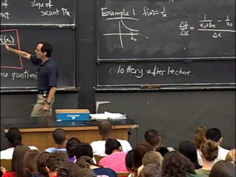
So let's do an example.

This example, we'll call this example one.

We'll take the function f(x) , which is 1/x .

That's sufficiently complicated to have an interesting answer,

and sufficiently straightforward that we can compute

the derivative fairly quickly.

So what is it that we're gonna do here?

All we're going to do is we're going to plug in this formula

here for that function.

That's all we're going to do, and visually

what we're accomplishing is somehow to take the hyperbola,

and take a point on the hyperbola,

and figure out some tangent line.

That's what we're accomplishing when we do that.

So we're accomplishing this geometrically

but we'll be doing it algebraically.

So first, we consider this difference delta f / delta x

and write out its formula.

So I have to have a place.

So I'm gonna make it again above this point x_0, which